As researchers we often want our collaborators to easily understand what we have done during an analysis. We could just share our raw data and code as it should be reproducible now you’ve completed module 3.1. It would be much better to create a reproducible report using RMarkdown that presents your code alongside its output (graphs, tables, etc.) with conventional text to explain it. Of course, reproducible reports aren’t just a useful way of sharing analyses with collaborators but can also act as a record for yourself.
Contents
3.2.3 Creating an RMarkdown Document
3.2.5 Code Chunks and Plain Text
3.2.1 What is RMarkdown?
Many programming languages used for data analysis have packages to generate reproducible reports - the most popular ones are Jupyter Notebooks for Python users and RMarkdown for R users. While both of these examples share many commonalities, their implementation and everyday applications differ.
RMarkdown is a file format (typically saved with the .Rmd extension) that can contain: a YAML header, text, code chunks, and inline code. The rmarkdown package converts this file into a report, most commonly into HTML or PDF. You don’t need to understand the multi-step process that rmarkdown uses to generate report outputs but for those interested please see here.
3.2.2 Installing RMarkdown
To use RMarkdown in RStudio you first need to install and load the rmarkdown package by running:
install.packages("rmarkdown")  # Installs package
library(rmarkdown)  # Loads package
3.2.3 Creating an RMarkdown Document
Now that you have rmarkdown installed let’s create a reproducible report! The first thing we need to do is create an RMarkdown file in RStudio:
- Click
File - Click
New File - Click
R Markdown
The following window will now appear:
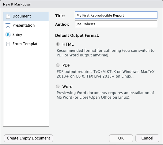
- Change the ‘Title’ to ‘My First Reproducible Report’ and the Author to your name
- Click
OK
You should now have a file that looks like this:
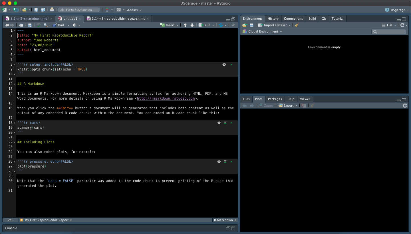
As you can see, newly created RMarkdown files come with some basic instructions and examples but we are not interested in these so select and delete them before saving your document. We can now populate our RMarkdown file with our own analyses and information.
3.2.4 YAML Header
YAML headers lives at the top of your RMarkdown file and are delineated by three dashes (—) at the top and at the bottom of it:
---
title: "My First Reproducible Report"
author: "Joe Roberts"
date: "15/06/2020"
output: html_document
---
YAML headers are optional but when you create a new RMarkdown file the title, author, date and output format are printed at the top of your document by default. Although this section is optional it is usually a good idea to include a YAML header as they can be used to specify:
- Document characteristics (e.g. title, authors, creation date, etc.)
- Pandoc arguments to specify output file information (e.g. file type, reference format, etc.)
Using the above code as an example, add a YAML header containing your title, author, date and output information to the RMarkdown file we just created:
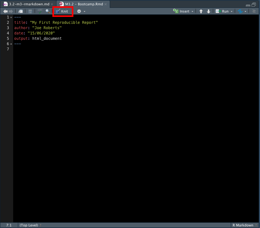
Now click knit to compile the .Rmd into a .html file (red box in the above image). RStudio will open a separate preview window to display the output of your .Rmd file and also save a .html file in the same folder as your .Rmd file. Your preview should look like this:
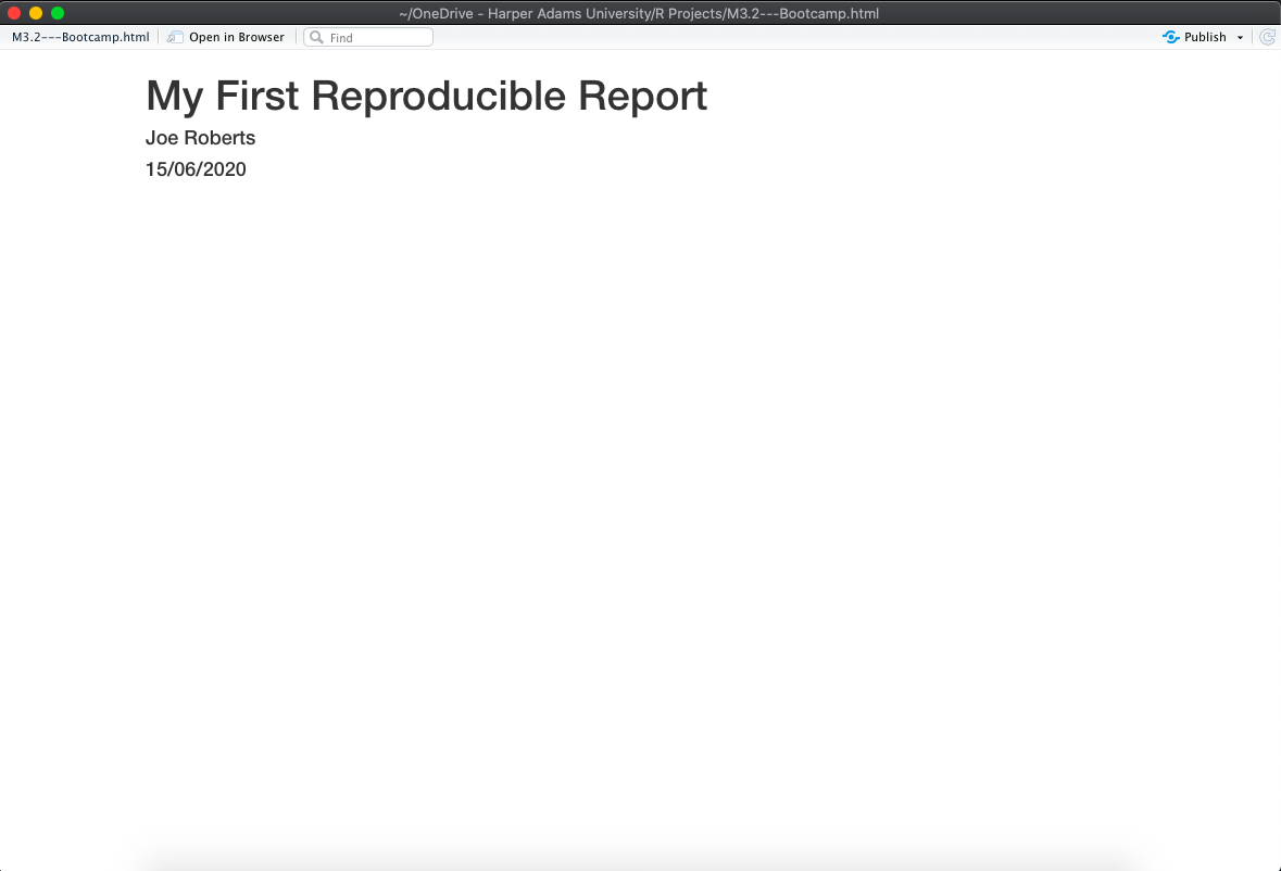
Congratulations - you’ve just compiled your first RMarkdown file! Below the YAML header is where we write code and text as well as displaying any outputs (e.g. plots, tables, etc.). Let’s take a closer look at these aspects of RMarkdown.
3.2.5 Code Chunks and Plain Text
Code chunks can be interspersed within the text of the report and are delineated by three backticks at the top and at the bottom. Top backticks are followed by curly brackets that specify the:
- Programming language
- Code chunk name (optional, but good practice)
knitroptions that control how the code, output, or figures are interpreted and displayed
Everything after the chunk name HAS to be a valid R expression! RMarkdown doesn’t pay attention to anything loaded in other R scripts or the global environment, you MUST load all objects and packages in the RMarkdown script.
```{r example-code-chunk, include = TRUE}
# This is an example code chunk
```
The above code chunk is specifies R as the programming language, that the chunk is called example-code-chunk and that it should be included in the RMarkdown .html document. Let’s add some plain text and a code chunk to our own RMarkdown file. Copy the following into your RMarkdown file and knit again:
This is our first code chunk:
```{r our-first-code-chunk, include = TRUE}
# Load the cars data into a new object
car_data <- cars

# Examine first five rows of this object
head(car_data)
```
There are lots of different knitr options availble to you to customise the behaviour of your code chunks. A summary of key options can be found here.
3.2.6 Plots
Inserting plots into an RMarkdown file is very easy! The more challenging aspect is adjusting their format using knitr options. First, insert a second code chunk into your RMarkdown file called example-plot-chunk and then create a plot by adding the following code and running knit:
# Create a plot of the car data
plot(car_data)
RMarkdown maximises plot height while keeping them within the margins of the page and maintaining aspect ratio. To manually set the figure dimensions, you can insert an instruction into the curly brackets:
```{r example-plot-chunk, fig.width = 10, fig.height = 5, include = TRUE}
plot(car_data)
```
Hopefully you now have two code chunks in your RMarkdown file.
3.2.7 Tables
R Markdown displays data frames and matrixes as they would be in the R terminal (in a monospaced font). If you prefer that data be displayed with additional formatting you can use the knitr::kable function:
# Create a dataframe
A <- c("a", "a", "b", "b")
B <- c(5, 10, 15, 20)
dataframe <- data.frame(A, B)

# Format using `kable` package
library(knitr)
kable(dataframe, digits = 2)
Insert the above code into a third data chunk in your RMarkdown file and knit. There are many alternative ways of creating tables in RMarkdown, which you can investigate yourself.
3.2.8 Markdown Basics
You can format the text in your RMarkdown file with Pandoc’s Markdown, a set of markup annotations for plain text files. When you compile your file, Pandoc transforms the marked up text into formatted text in your final file format. Markdown formatting examples:
- italics =
*italics* - bold =
**bold** - links =
[links](https://rmarkdown.rstudio.com/lesson-8.html)
A comprehensive reference guide to Markdown formatting can be found here.