Analysing data using R can generate complex scripts that might make sense to you while you’re actively working on them, but they won’t to future you or collaborators. This bootcamp module offers guidance to improve the reproducibility of your code for yourself and others. Following this guidance will also improve your R workflow and reduce errors.

SCRIPT - Use this for the practice exercises below

Contents

3.1.1 Styling Your Code

3.1.2 RStudio Addins

3.1.3 Project Organisation

3.1.4 RStudio Projects

3.1.5 Practice Exercises

3.1.1 Styling Your Code

“Good coding style is like correct punctuation: you can manage without it, butitsuremakesthingseasiertoread.” - Hadley Wickham

As we saw in module 1.1 of the bootcamp, it is important to give your R scripts structure to make them human-readable. We can take this one step further by styling our code to meet a set of “rules” to improve its reproducibility. There are lots of different styles but we will use Hadley Wickham’s guide. This module outlines the basics of code styling, for a more comprehensive overview please see here.

Naming files and objects

Selecting good names for files and objects may seem easy, but isn’t! Whatever you do, try to avoid the obvious - e.g. naming plots plot1, plot2, etc. Use the following naming rules and you won’t go wrong!

File names

• Make them meaningful
• Avoid spaces and unusual characters
• Use lowercase letters

# Good
aphid_mortality_analysis_2019.R

# Bad
Script +2.R  

Object names

• Use underscores to separate words
• Make names informative but short
• Do not reuse names within an analysis
• Avoid using names of functions
• Variable names == nouns while function names == verbs

# Good
mean_aphid_mortality

# Bad
mean.aphid.mortality
MeanAphidMortality
mam
aphid_Mortality

Spacing

Commas

• Always put a space after a comma:

# Good
x[, 1]

# Bad
x[,1]
x[ ,1]
x[ , 1]

Parentheses

• Do not put spaces inside or outside () for regular function calls:

# Good
mean(x, na.rm = TRUE)

# Bad
mean (x, na.rm = TRUE)
mean( x, na.rm = TRUE )

• Place a space before and after () when used with if, for, or while:

# Good
if (debug) {
  show(x)
}

# Bad
if(debug){
  show(x)
}

• Place a space after () used for function arguments:

# Good
function(x) {}

# Bad
function (x) {}
function(x){}

Infix operators

• Most infix operators (==, +, -, <-, etc.) should always be surrounded by spaces:

# Good
height <- (feet * 12) + inches
mean(x, na.rm = TRUE)

# Bad
height<-feet*12+inches
mean(x, na.rm=TRUE)

• However, operators with high precedence: ::, :::, $, ^, : etc. should NOT have spaces:

# Good
sqrt(x^2 + y^2)
df$z
x <- 1:10

# Bad
sqrt(x ^ 2 + y ^ 2)
df $ z
x <- 1 : 10

Assignment

• Use <- not =:

# Good
x <- 1:10

# Bad
x = 1:10

• Avoid assignment in function calls:

# Good
x <- complicated_function()
if (nzchar(x) < 1) {
  # do something
}

# Bad
if (nzchar(x <- complicated_function()) < 1) {
  # do something
}

Long lines

Try to limit your code to 80 characters per line as this fits comfortably on a printed page with a reasonably sized font. How do you know when you’ve reached 80 characters? RStudio has the option to include a margin in your script, which you can activate by:

1. Click tools in the menu
2. Click global options
3. Click code
4. Click display
5. Click show margin

If a function call is too long to fit on a single line, use one line each for the function name, each argument, and the closing ). This helps make the code easier to read and to change later.

# Good
do_something_very_complicated(
  something = "that",
  requires = many,
  arguments = "some of which may be long"
)

# Bad
do_something_very_complicated("that", requires, many, arguments,
                              "some of which may be long"
                              )

3.1.2 Styling Your Code With RStudio Addins

RStudio Addins provide extra functionality through a point and click menu. Install addins by running:

install.packages('addinslist')

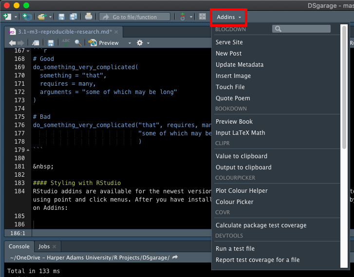
After you have installed addins, you can access them by clicking on Addins:

However, before you can style your code using addins you will need to install the styler package:

install.package('styler')

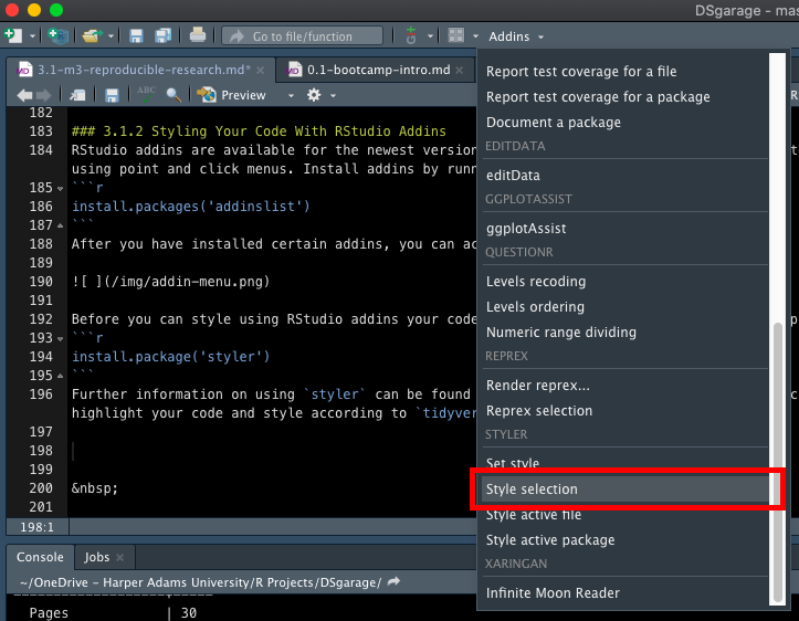
Further information on using styler can be found here. You can now highlight your code and style to tidyverse formatting by selecting style selection in the styler section of the addins menu:

3.1.3 Project Organisation

Most projects begin as a seemingly random collection of files and many people end up organising their projects like this:

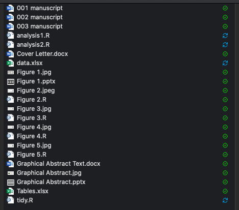
This is not a well organised project as it is confusing, mixes up many file types and modifies the original data file. Why organise your projects better?

• Ensures data integrity
• Simplifies code sharing
• Promotes reproducibility

Truly reproducible research requires self-contained projects, where all should be contained within a single folder. I recommend that you create a folder called repos/ that you save your project folders in, e.g. C:/User/owner/Documents/repos/proj/. This ensures your project folders are neatly separated from other files and will be useful when we explore Git in a later module.

Once you have a repos/ folder, you can create a project folder. The following structure is what I find works for me but you may want to find a variation of it that works for you. If you do modify this structure it is important to remember that the basic premise of keeping repositories self-contained should remain!

C:/
└── Documents/
    └── repos/
        └── proj/
            ├── data/
            ├── docs/
            ├── figs/
            ├── funs/
            ├── out/
            ├── data_cleaning.R
            └── data_analysis.R

The project repository contains separate directories that can be used to store different file types. Our data_analysis and data_cleaning files are stored in the project root, allowing easy use of relative paths over explicit paths e.g.read.csv(here('data', 'data_file.csv')) rather than read.csv('C:/Users/owner/Documents/repos/my_project/data/data_file.csv'). Relative paths are preferable because they allow projects to be used by multiple people without the need to re-write code. If you use explicit paths and change computer, or the project is opened by another person, the code will break as they will not have the same directory structure as the computer that the code was created on.

Note: the example above used an R package called here_here, calling the function here(). I highly recommend you invest time in learning to use this useful package, which can be found here.

data/

Treat your data as read-only! Data is typically time consuming and/or expensive to collect. Working with your raw data interactively (e.g. in Excel) where they it be modified means you are never sure of where the data came from, or how it has been modified since collection. This can cause all sorts of problems later.

• docs/: contains the output documents
• funs/: contains custom functions you write
• out/: contains files that are produced from the original data e.g. cleaned data files
• figs/: contains figures generated from your scripts

All output can be treated as disposable as it could be easily regenerated by running the code.

3.1.4 RStudio Projects

There are a number of tools and packages that can help you manage your work effectively. RStudio has incredible project management functionality in-built, so make sure you exploit this. When using RStudio projects, all of your data, plots and scripts are located in a relative path in relation to the base directory you create when setting up the project. This makes them very easy to access without having to set your working directory. Detailed guidance on using RStudio projects can be found here.

3.1.5 Practice Exercises

1 Install RSudio Addins and the styler package by running:

install.packages('addinslist')
install.packages('styler')

Download the script above, open it with RStudio and convert it to tidyverse style using styler.

2 Create an RStudio project following these instructions:

1. Click the File menu button, then New Project
2. Click New Directory
3. Click New Project
4. Type in the name of the directory to store your project e.g. my_project
5. Click the Create Project button