Correlation
SCRIPT 2.3 Use this to follow along on this page and for the Practice exercises below.
Overview
Most of you will have heard the maxim “correlation does not imply causation”. Just because two variables have a statistical relationship with each other does not mean that one is responsible for the other. For instance, ice cream sales and forest fires are correlated because both occur more often in the summer heat. But there is no causation; you don’t light a patch of the Montana brush on fire when you buy a pint of Haagan-Dazs. - Nate Silver
Correlation is used in many applications and is a basic tool in the data science toolbox. We use it to to describe, and sometimes to test, the relationship between two numeric variables, principally to ask whether there is or is not a relationship between the variables (and if there is, whether they tend to vary positively (both tend to increase in value) or negatively (one tends to decrease as the other increases).
Contents
2.3.1 The question of correlation
2.3.1 The question of correlation
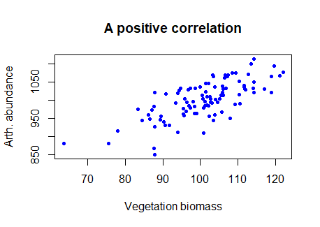
The question of correlation is simply whether there is a demonstrable association between two numeric variables. For example, we might wonder this for two numeric variables, such as a measure of vegetation biomass and a measure of insect abundance. Digging a little deeper, we are interested in seeing and quantifying whether and how the variables may “co-vary” (i.e, exhibit significant covariance). This covariance may be quantified as being either positive or negative and may vary in strength from zero, to perfect positive or negative correlation (+1, or -1). We traditionally visualise correlation with a scatterplot (plot() in R). If there is a relationship, the degree of “scatter” is related to strength of the correlation (more scatter = a weaker correlation).
E.g., we can see in the figure below that the two variables tend to increase with each other positively, suggesting a positive correlation.
# Try this:

# Flash challenge
# Take the data input below and try to exactly recreate the figure above!

veg <- c(101.7, 101.2, 97.1, 92.4, 91, 99.4, 104.2, 115.9, 91.9, 101.4,
93.5, 87.2, 89.2, 92.8, 103.1, 116.4, 95.2, 80.9, 94.9, 88.8,
108.2, 86.1, 104.1, 101.5, 116.9, 109.6, 103.7, 83.9, 85.9, 88.5,
98.9, 98.8, 107.8, 86.5, 92.6, 76, 95.2, 105.3, 103.1, 89.3,
100.1, 103.1, 87.7, 92.4, 91.5, 105.4, 105.7, 90.5, 105.6, 101.6,
97.4, 93.4, 88.7, 81.1, 100.9, 91.6, 102.4, 92.8, 92, 97.1, 91.1,
97.3, 104, 99, 101.5, 112.8, 82.4, 84.9, 116.3, 92.2, 106.2,
94.2, 89.6, 108.8, 106.2, 91, 95.5, 99.1, 111.6, 124.1, 100.8,
117.6, 118.6, 115.8, 102.2, 107.7, 105, 86.7, 99, 101.8, 106.3,
100.3, 86.6, 106.4, 92.6, 108.2, 100.5, 100.9, 116.4)

arth <- c(1002, 1006, 930, 893, 963, 998, 1071, 1052, 997, 1044, 923,
988, 1022, 975, 1022, 1050, 929, 928, 1019, 957, 1054, 850, 1084,
995, 1065, 1039, 1009, 945, 995, 967, 916, 998, 988, 956, 975,
910, 954, 1044, 1063, 948, 966, 1037, 976, 979, 969, 1009, 1076,
943, 1024, 1071, 969, 963, 1020, 936, 1004, 961, 1089, 953, 1037,
962, 977, 958, 944, 933, 970, 1036, 960, 912, 978, 967, 1035,
959, 831, 1016, 901, 1010, 1072, 1019, 996, 1122, 1029, 1047,
1132, 996, 979, 994, 970, 976, 997, 950, 1002, 1003, 982, 1071,
959, 976, 1011, 1032, 1024)
2.3.2 Data and assumptions
Pearson correlation
“Traditional correlation” is sometimes referred to as the Pearson correlation. The data and assumptions are important for the Pearson correlation - we use this when there is a linear relationship between our variables of interest, and the numeric values are Guassian distributed.
More technically, the Pearson correlation coefficient is the covariance of two variables, divided by the product of their standard deviations:
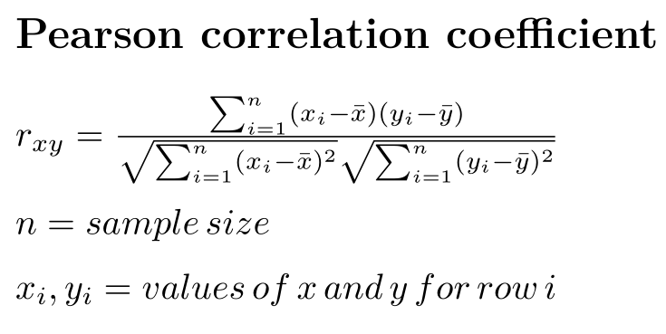
The correlation coefficient can be calculated in R using the cor() function.
# Try this:
# use veg and arth from above

# r the "hard way"

# r = ((covariance of x,y) / (std dev x * std dev y) )


# sample covariance (hard way)
(cov_veg_arth <- sum( (veg-mean(veg))*(arth-mean(arth))) / (length(veg) - 1 ))

cov(veg,arth) # easy way

# r the "hard way"
(r_arth_veg <- cov_veg_arth / (sd(veg) * sd(arth)))

# r the easy way
help(cor)
cor(x = veg, y = arth,
    method = "pearson") # NB "pearson" is the default method if unspecified
2.3.3 Graphing
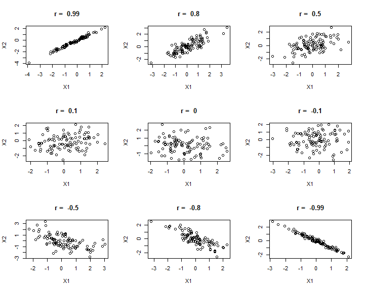
We can look at a range of different correlation magnitudes, to think about dignosing correlation.
If we really care and value making a correlation between 2 specific variables, traditionally we would use the scatterplot like above with the veg and arth data, and the calculation of the correlation coefficient (using plot() and cor() respectively). On the other hand, we might have loads of variables and just want to quickly assess the degree of correlation and intercorrelation. To do this we might just make and print a matric of the correlation plot (using pairs()) and the correlation matrix (again using cor())
## Correlation matrices ####
# Try this:

# Use the iris data to look at correlation matrix
# of flower measures
data(iris)
names(iris)
cor(iris[ , 1:4]) # all rows, just the numeric columns

# fix the decimal output
round(cor(iris[ , 1:4]), 2) # nicer

# pairs plot
pairs(iris[ , 1:4], pch = 16,
      col = iris$Species) # Set color to species...
R output
> round(cor(iris[ , 1:4]), 2) # nicer
             Sepal.Length Sepal.Width Petal.Length Petal.Width
Sepal.Length         1.00       -0.12         0.87        0.82
Sepal.Width         -0.12        1.00        -0.43       -0.37
Petal.Length         0.87       -0.43         1.00        0.96
Petal.Width          0.82       -0.37         0.96        1.00
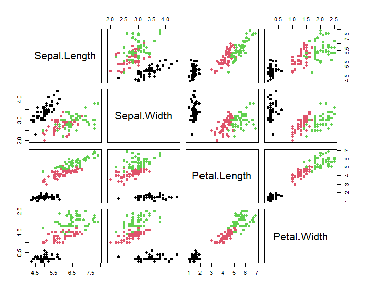
In this case, we can see that the correlation of plant parts is very strongly influenced by species! For further exploration we would definitely want to explore and address that, thus here we have shown how powerful the combination of statistical summary and graphing can be.
2.3.4 Test and alternatives
We may want to perform a statistical test to determine whether a correlation coefficient is “significantly” different to zero, using Null Hypothesis Significance Testing. There are a lot of options, but a simple solution is to use the cor.test() function.
An alternative to the Pearson correlation (the traditionl correlation, assuming the variables in question are Gaussian), is the Spearman rank correlation, which can be used when the assumptions for the Pearson correlation are not met. We will briefly perform both tests.
See here for further information on Pearson correlation
See here for further information on Spearman rank correlation
Briefly, the principle assumptions of the Pearson correlation are:
-
The relationship between the variables is linear (i.e., not a curved relationship)
-
The variables exhibit a bivariate Gaussian distribution (in pactice, it is often accepted that each variable is Gaussian)
-
Homoscedasticity (i.e., the variance is similar across the range of the variables)
-
Observations are independent
-
Absence of outliers
Further practical information about correlation
Let’s try a statistical test of correlation. We need to keep in mind an order of operation for statistical analysis, e.g.:
1 Question
2 Graph
3 Test
4 Validate (e.g. test assumptions)
## Correlation test ####
# Try this:

# 1 Question: whether Petal length and width are correlated

# 2 Graph
plot(iris$Petal.Width, iris$Petal.Length,
     xlab = "Petal width",
     ylab = "Petal length",
     col = iris$Species, pch = 16)

# 3 Test
cor.test(iris$Petal.Width, iris$Petal.Length)
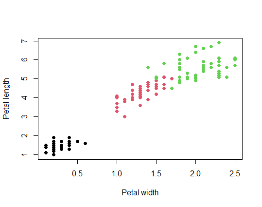
R output
> cor.test(iris$Petal.Width, iris$Petal.Length)

	Pearson's product-moment correlation

data:  iris$Petal.Width and iris$Petal.Length
t = 43.387, df = 148, p-value < 2.2e-16
alternative hypothesis: true correlation is not equal to 0
95 percent confidence interval:
 0.9490525 0.9729853
sample estimates:
      cor
0.9628654
Note about results and reporting
When we do report or document the results of an analysis, we we would do it in different ways depending on the intended audience.
Documenting results only for ourselves
It would be typical to just comment the R script and have your script and data file in fully reproducible format. This format would also work for close colleague (who also use R), or collaborators, to use to share or develop the analysis. Even in this format, care should be taken to clean up redundant or unnecessary code, and to organize the script as much as possible in a logical way, e.g. by pairing graphs with relevant analysis outputs, removing analyses that were tried but obsolete (e.g. because a better analysis was found), etc.
Documenting results to summarize to others
Here it would be typical to summarize and format output results and figures in a way that is most easy to consume for the intended audience. There should NEVER BE RAW COPIED AND PASTED STATISTICAL RESULTS (omg!). A good way to do this would be to use R Markdown to format your script to produce an attractive summary, in html, MS Word, or pdf formats (amongst others). Second best (primarily because it is more work and harder to edit or update) would be to format results in word processed document (like pdf, Word, etc.).
Statistical summary
Most statistical tests under NHST will have 3 quantities reported for each test: the test statistic (different for each test, “r” for Pearson correlation), the sample size or degrees of freedom, and the p-value. For our results above, it might be something like:
We found a significant correlation between petal width and length (Pearson’s r = 0.96, df = 148, P < 0.0001)
NB the rounding of decimal accuracy, and the formatting of the p-value. The 95% confidence interval of the estimate of r is also produced (remember, we are making an inference on the greater population from which our sample was drawn), and we might also report that in our descriptive summary of results, if it is deemed important.
# 4 Validate
hist(iris$Petal.Length) # Ummm..
hist(iris$Petal.Width) # Yuck

# We violate the assumption of Gaussian

# ... Relatedly, we also violate the assumption of independence
# due to similarities within and differences between species!
Flash challenge
Write a script following the steps to question, graph, test, and validate for each iris species separately. Do these test validate? How does the estimate of correlation compare amongst the species?
Correlation alternatives to Pearson’s
There are several alternative correlation estiamte frameworks to the Pearson’s; we will briefly look at the application of the Spearman correlation. THe main difference isa relaxation of assumptions. Here the main assumption is that:
-
The data are ranked or otherwise ordered
-
The data rows are independent
Hence, rank Spearman rank correlation descriptive cefficient and test are appropriate even if the data are not bivariate Gaussian or if the data are not strictly linear in their relationship.
# Spearman rank correlation ####

# Try this:

height <- c(18.4, 3.2, 6.4, 3.6, 13.2, 3.6, 15, 5.9, 13.5, 10.8, 9.7, 10.9,
18.8, 11.6, 9.8, 14.4, 19.6, 14.7, 10, 16.8, 18.2, 16.9, 19.8,
18.2, 2.6, 18.8, 8.4, 18.9, 9.5, 19)

vol <- c(16.7, 17.8, 17.9, 21.1, 21.2, 21.4, 23.2, 25.7, 26.1, 26.4,
26.8, 27, 27.8, 28.2, 28.5, 28.6, 28.7, 29.1, 30.2, 31, 32.3,
32.3, 32.5, 33.2, 33.5, 33.8, 35.2, 36.1, 36.6, 39.5)

plot(height, vol,
     xlab = "Height",
     ylab = "Volume",
     pch = 16, col = "blue", cex = .7)

# Spearman coefficient
cor(height, vol, method = "spearman")

# Spearman test
cor.test(height, vol, method = "spearman")

R output
> cor(height, vol, method = "spearman")
[1] 0.3945026

> cor.test(height, vol, method = "spearman")

	Spearmans rank correlation rho

data:  height and vol
S = 2721.7, p-value = 0.03098
alternative hypothesis: true rho is not equal to 0
sample estimates:
      rho
0.3945026
NB the correlation coefficient for the Spearman rank coprrelation is notated as “rho” (the Greek letter), reported and interpreted exactly like the Pearson correlation coefficient, r.
2.3.5 Practice exercises
For the following exercises, use 2 datasets: the waders data from the package {MASS}, and the cape furs dataset cfseals you can download here
1 Load the waders data and read the help page. Use the pairs function on the data and make a statement about the overall degree of intercorrelation between variables based on the graphical output.
2 Think about the variables and data themselves in waders. Do you expect the data to be Gaussian? Formulate hypothesis statements for correlations amongst the first 3 columns of bird species in the dataset. Show the code to make 3 good graphs (i.e., one for each pairwise comparison for the first 3 columns), and perform the 3 correlation tests.
3 Validate the test performed in question 2. Which form of correlation was performed, and why. Show the code for any diagnostic tests performed, and any adjustment to the analysis required. Formally report the results of your validated results.
4 Load the 2.3-cfseal.xlsx data and examine the information in the data dictionary. Analyse the correlations amongst the weight heart and lung variables, utilising the 1 question, 2 graph, 3 test and 4 validate workflow. Show your code and briefly report the results.
5 Comment on the expectation of Gaussian for the age variable in the cfseal data. WOuld expect this variable to be Gaussian? Briefly explain you answer and analyse the correlation between weight and age, using our 4 step workflow and briefly report your results.
6 Write a plausible practice question involving any aspect of the use of correlation, and our woprkflow. Make use of the data from either the waders data, or else the cfseal data.